Google Sheets Power User Tips

A lot of hardcore Excel users scoff at Google Sheets, but I find it to be a fantastic and powerful spreadsheet app with superb collaboration tools. I often see people failing to take full advantage of the power of Google Sheets, or sometimes even the basic features, so hopefully these tips will help.

Table of Contents

• Freeze Rows and Columns
• Filter Views
• Conditional Formatting with Functions across Columns
• Use Named Functions
• Add Slicers For Pivot Tables Or Charts
• Snoop on users of your docs/sheets

Freeze Rows and Columns

Freezing rows and/or columns allows those rows/columns to remain visible even if you scroll down or sideways, making it much easier for your users to navigate a sheet. This may seem basic to some of you, but I have seen a lot of Google sheets and this is not universally understood. Truthfully, huge spreadsheets without frozen rows/columns are a pet peeve of mine, so I had to list it first.

Use the View > Freeze menu item or just drag the thick gray bar that is visible in the gutter.

Filter Views

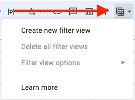
Instead of filtering the data for everyone, you can create a view of the data that only applies to people who select that view and does not affect the default view of the data.

Filter views work just like normal filters, except you can create multiple different views and give them human readable labels. The best part is that filter views update the URL, so you can bookmark a filter view or send someone a link to a filter view and they’ll see the data filtered just the way you want.

Conditional Formatting with Functions across Columns

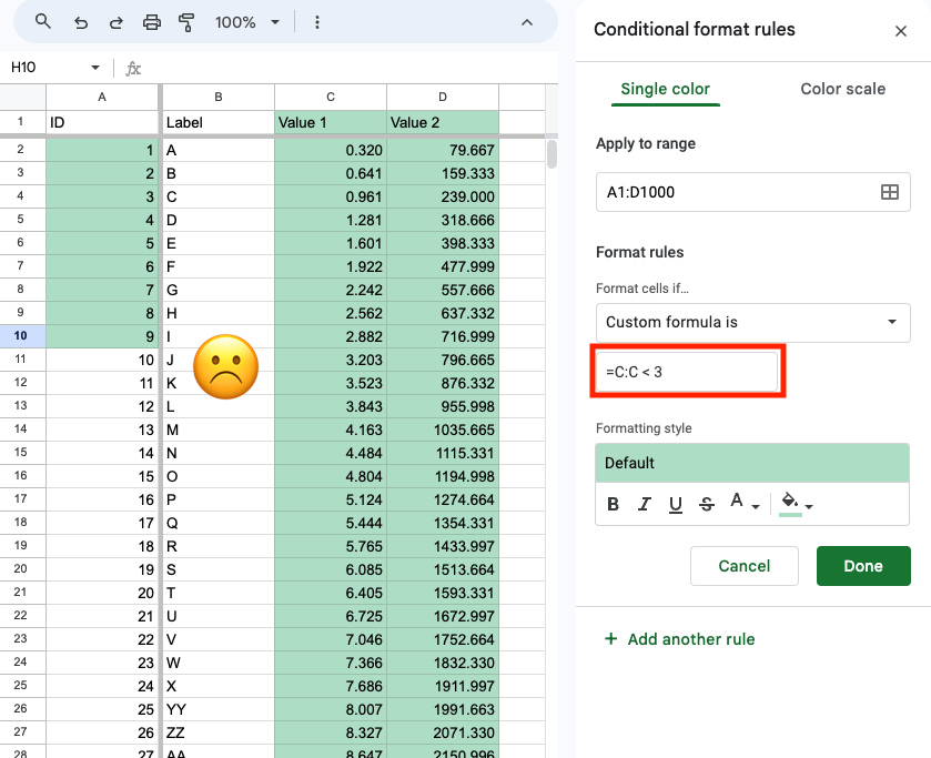
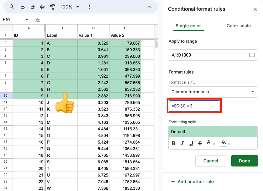
If you want to apply formatting (highlighting, colors, etc) based on a formula, you can use the “Custom formal” setting in Conditional format rules. Note that to apply evenly across columns, you will need to use dollar sign ($) syntax. See examples below:

Not using $ syntax means that for column A, it will apply where column C matches the formula, but for column B it will look at column D, and for column C it will look at column E, etc. That’s prob not what you want:

If you use $ syntax, then each column will be formatted based on the value in column C.

Use Named Functions

If you find yourself reusing complicated formulas, consider turning them into a custom Named Function.

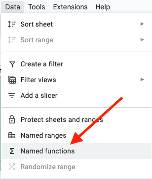
Pro tip: you can collect formulas you use often in different sheets into a single sheet and then import them into other sheets as needed.

Add Slicers For Pivot Tables Or Charts

If you create a pivot table and/or a chart, you can add a way for users to filter the data by adding a Slicer.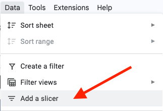

This makes it easy for your users to filter the data on your custom dashboards.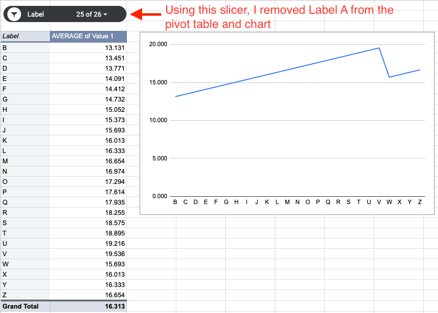

Snoop on users of your docs/sheets

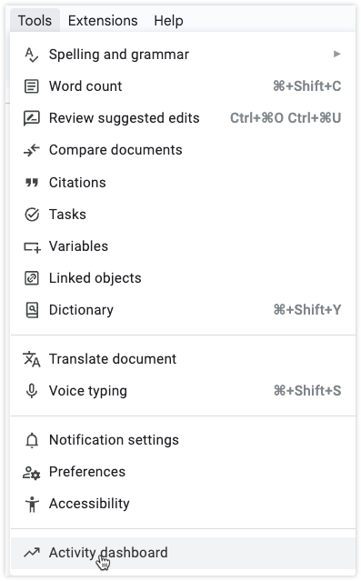
You can check who is viewing your document. Click Tools > Activity Dashboard

This will give you a view like this with different viewer analytics about your doc.

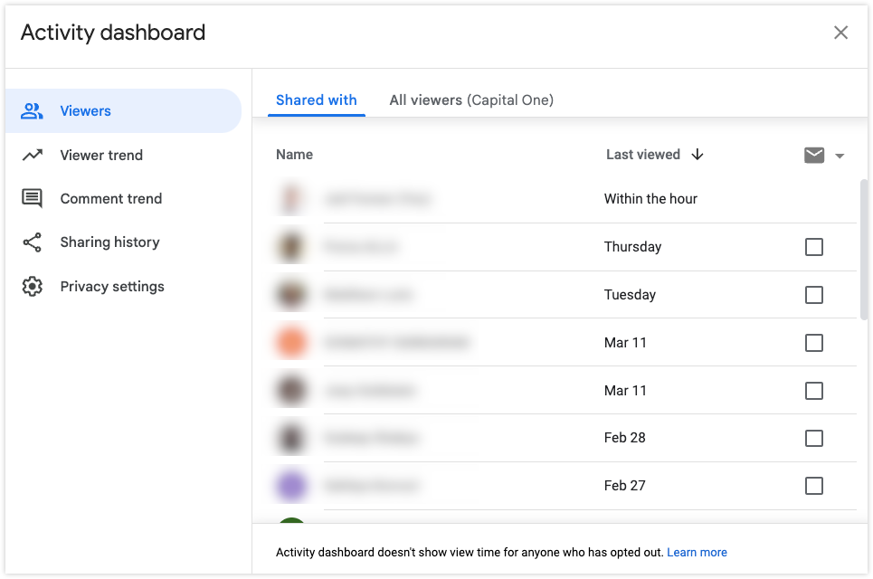
This tip works for Google Docs as well as Sheets.

You can also get notified when anyone edits your document

1. Go to Tools > Notifications Settings (In Sheets, you have to select the additional “Edit Notifications” item).
2. Select whether you want to be notified if someone adds or removes content from the doc.

Sneaky!